In this post, I will be going over some basic concepts in ElectroDynamics. The objective is to build up the prior knowledge required to understand COSMO (“COnductor-like Screening MOdel”) solvation models. I hope that this series of posts can be helpful to those who are getting into the world of quantum chemistry with an engineering mindset.

Dielectrics

---

Most matter are categorized as either conductors or insulators. Conductors have an abundance of electrons that float freely through the material. A typical metal has one or two electrons per atom shared all across. Conversely, insulators (or dielectrics) have their electrons on leashes. Instead, the electrons make microscopic displacements within the atom or molecule once subjected to an electric field.

Induced Dipoles

If we place a neutral atom in an electric field, our intuition will lead us to believe that the cloud of electrons would be displaced by a certain distance from its origin, leaving the atom polarized. A better way to illustrate this concept would be to consider the following rudimental model of an atom. It consists of a point nucleus (\(+q\)) surrounded by a uniformly charged spherical cloud (\(-q\)) of radius \(a\). The electron cloud is not limited to the surface of the sphere it also includes the body of the sphere. When \(E\) is applied, the neucleus moves with the field to the right by a distance \(d\). At equilibrium, the external field \(E\) pushing the neucleus to the right exactly balances the internal field pulling it to the left created by the cloud of electrons \(E_e\).

Fig. 1

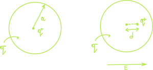
At equilibrium, \(E = E_e\). Now the field at a distance \(d\) from the center of a uniformly charged sphere is:

\[\begin{align} E_e = \frac{1}{4\pi\epsilon_0} \frac{qd}{a^3} \label{eq1}\tag{1} \end{align}\]

Equation \(\ref{eq1}\) is deduced in more details in the following post by appying Gauss’s law to find the electric field inside a uniformly charged sphere. Assuming the equation is correct, we have at equilibrium:

$$ E = \frac{1}{4\pi\epsilon_0} \frac{qd}{a^3} $$ or $$p = qd = (4\pi\epsilon_{0}a^3)E $$

The atomic polarizability is therefore

\[\alpha = 4\pi\epsilon_{0}a^3 = 3\epsilon_{0}v\]

where \(v\) is the volume of the atom. This is a crude approximation but it is accurate to within a factor of four or so for many simple atoms.

Polarizability is a tendency of matter, when subjected to an electric field, to acquire an electric dipole moment (\(p\) above) in proportion to that applied field. This is a key property of the solvent that is used in the COSMO solvation models. We will now explore polar molecules in the later section. Polar molecules have built-in permanent dipole moments which cannot be induced like the \(H_{2}O\) molecule a very common polar solvent.

Polar Molecules

References

1. MLA. Griffiths, David J. (David Jeffery), 1942-. Introduction to Electrodynamics. Boston :Pearson, 2013.